Hyperparameter optimization is one of the most difficult problems in machine learning. How many layers should my neural network be? How many kernels should each layer have? What type of activation function should I use? What value should I set as my learning rate?
In the month of August, I became obsessed with this problem – how to optimize hyper-parameters. I started creating an open-source tool called Hypermax, available for free through Python’s “pip install” command, or directly from the latest source code on Github (https://github.com/electricbrainio/hypermax). Initially, the tool was just there to do some surrounding non-core stuff, such as monitor the execution time and RAM usage of models, and to generate graphs based on the results of the trials. The core algorithm was not my own – it was simply the TPE algorithm, as implemented in the Hyperopt library. Originally, Hypermax was just intended to make optimization more convenient.
But I quickly became obsessed with this idea of how to make a better optimizer. TPE was an industry leading algorithm. Although invented in 2012-2013, it was still being cited as recently as 2018 as one of the best algorithms for hyperparameter optimization. In most cases, it was the leading algorithm, but more recently there have been a few new approaches, like SMAC, which can do just as well in general, but not clearly better in all cases. Even more recently (July 2018), there has been work on this algorithm called Hyperband, and its evolved version, BOHB (which is just a combination of Hyperband and TPE). However, TPE is still an industry leading algorithm, with top-notch general case performance across a wide variety of optimization problems. It has also been well validated by many people who have used it across many machine learning algorithms and proven its effectiveness. It is for this reason that we decided to use it as the basis of our research. Our goal was to make an improved version of TPE.
We started our research by testing various ways that TPE can be manipulated in order to improve its results, and various ways that we could gather data in order to know what works. This formed the basis of the first version of our Adaptive-TPE algorithm. This first research was great, and validated that we were onto something, both in terms of our approach to researching a better TPE, and in the specific techniques that we used to improve it. In that research, 4 of the 7 things we tried improved TPE. The other 3 things we tried had absolutely no impact on the results (neither worse or better).
In this article, we will discuss version two of our Adaptive-TPE algorithm. Version 2 takes our approach to a whole new level. We are repeating a basic description of our approach in this article so that you don’t have to read the original research. However, it will be condensed.
Levers for Improving TPE
TPE (Tree of Parzen Estimators), and the Hyperopt implementation of it, don’t have a whole lot of hyperparameters that we can try to tune. But it does have a few. Additionally, there are algorithmic things we can do to mess with the algorithm and see if we get better results.
We can think of TPE as being an algorithm which takes a history of trials, and predicts the best trial to test next. TPE itself has a single primary hyper-parameter, gamma. But we can manipulate the data it uses as input in a variety of ways. We can also provide weights to the trials inside the TPE algorithm. We can change our loss function, which might alter the way that TPE behaves. Additionally, there’s a couple hypothetical ways we could manipulate TPE – we could force TPE to spend more time exploring certain hyper-parameters by ‘locking in’ the values for the others for some trials. Additionally, we could have separate TPE distributions for separate hyper-parameters, even while they are being optimized jointly. This may sound crazy but there is some underlying motivation for this if those hyper-parameters are highly independent of one another. So overall, our landscape for improving the TPE algorithm looks like this:
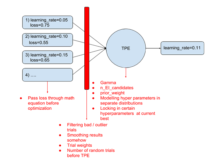
In our first round of ATPE research, we tested 7 of these techniques for improving TPE. We were able to validate 4 techniques that improved TPE:
- Pass loss through math equation before optimization (failed)
- Number of random trials before TPE (success)
- Tuning Gamma (success)
- Tuning n_EI_candidates (success)
- Tuning prior_weight (failure)
- Modelling hyper-parameters in separate distributions (failed)
- Locking in certain hyperparameters at current best value (success)
Additionally, in the original paper, they tested the “Trial Weights” technique and already validated that it improves results. We were unable to dissect the Hyperopt code enough to get Trial Weights working ourselves. However, filtering trials has a similar the same effect as weighting them (since trial weights was only used to down-weight old trials). The only difference is that there is a bit more stochasticism involved in filtering, and weighting would have likely been more smooth and consistent. So ultimately we decided to include filtering despite not validating it in our original research.
In addition, because of the success of the parameter locking (also called Bagged Optimization in our original paper), we wanted to expand upon the ways that parameters could be locked, to give options for our ATPE algorithm. We made several adjustments to parameter locking compared to the first ATPE algorithm:
- We expanded the algorithm to allow locking parameters both to top performing results or to a random value from anywhere in that parameters range, e.g. random search that parameter
- When locking to a top performing result, we allow locking not just to the current best, but to any result within the top K percentile of results
- When choosing the cutoff point for which parameters to lock, we multiply the correlations by an exponent, which alters the distribution of correlations to have more or less bias towards the larger numbers
- We allow the algorithm to choose either high correlated parameters or low correlated when selecting the cutoff point, e.g. it might choose to lock the 50% highest correlated parameters or the 50% lowest correlated parameters. Previously only highly correlated parameters would be locked first.
- When deciding whether to lock a parameters, we allow the probability to vary from a 50-50 chance. We have two different modes for choosing the probability – either a fixed probability, or a probability determined based on multiplying the parameters correlation by a factor C
The idea in general was to give the algorithm a variety of ways to explore more tightly or more widely depending on what the circumstances are.
So ultimately, our ATPE algorithm looks roughly like the following:
- Compute Spearman correlations for each hyperparameter, raise to an exponent
- Determine a cutoff point between correlated and uncorrelated parameters based on the cumulative correlation. The parameters can be sorted in either direction, with correlated ones first or uncorrelated ones first
- For parameters that are chosen for potential locking, they have a random chance of being locked in that round. The probability varies by depending on the mode for that round: – In fixed probability mode, there is a fixed chance that this parameter will be locked, varying from 20% to 80% – In correlation probability mode, the chance of locking this parameter is chosen by multiplying the correlation by a factor C
- We assign the locked values depending on what mode ATPE is in: – If the ATPE mode is in random-locking mode, then for parameters that are chosen to be locked, we assign them a random-value from anywhere in their search space – If the ATPE mode is in top-locking mode, then we choose a single top performing result from the result-history. The top performing result may not be the current best, but is chosen from the top K percentile of results for that round. All parameters chosen for locking are then locked to the same value they had in that top-performing result.
- We create an alternative result history which has some results filtered out randomly according to the filtering mode for this round: – If the filtering mode is Age, then we randomly filter out results based on their age within the result history. We use their position within the result history (0 to 1 where 0 is the first result and 1 is the most recent), and multiply that position by a factor F which determines the probability that the result will be kept. We randomly determine if the result will be kept using that probability. This creates a bias towards keeping more recent results, with more or less filtering controllable by factor F – If the filtering mode is Loss_Rank, then we randomly filter out results based on the ranking of their losses. The mechanism is similar to Age filtering, except the results have been sorted by their losses first. – If the filtering mode is Random, then all results have an equal likelihood of being filtered out, with probability P – If filtering mode is None, then we do not perform any filtering and retain all results in the history – Only the TPE algorithm receives the filtered result history. The statistics and locking are always computed based on the full history.
- Lastly, we use the magical Bayesian math of the TPE algorithm to predict the remaining parameters that have not been locked: – We provide the TPE algorithm the values for the parameters that have been locked. This allows it to perform partial-sampling – e.g. it will predict good values for the remaining parameters, given the values for the locked ones.
All in all, this is an optimization algorithm with the Bayesian math of the TPE algorithm at its core. It has simply been surrounded with two additional mechanisms – one to filter the results fed into the TPE algorithm, and the other is to only use TPE for a subset of parameters at a time, while locking the remaining ones using the mechanism described above. TPE still uses its magic to predict the remaining parameters given the values of the locked ones.
The algorithm appears to have a lot of potential, but implementing it introduces a new problem: How do you choose ATPE’s own parameters at each round? It itself has a bunch of parameters that have to vary as it gains new information. They are described here with their actual variable names in the code:
- resultFilteringMode: Age, LossRank, Random, or None
- resultFilteringAgeMultiplier: For Age filtering, the multiplier applied to the results position in history to determine the probability of keeping that result
- resultFilteringLossRankMultiplier: For Loss filtering, the multiplier applied to the rank of the result when sorted by loss, used to determine the probability of keeping that result
- resultFilteringRandomProbability: For Random filtering, the probability of keeping any given result
- secondaryCorrelationExponent: This is the exponent that correlations are raised by when determining which parameters to lock and which ones to explore with TPE. Varies between 1.0 and 3.0
- secondaryCutoff: When choosing which parameters to consider for locking, this is the cutoff point of cumulative correlation that is used to determine the parameters to be locked. Varies between -1.0 and 1.0. Negative numbers are used to indicate a reverse sorting, where low-correlated variables are locked first. Positive numbers indicate that high-correlated variables should be locked first.
- secondaryLockingMode: Either Top or Random, determines whether we explore tightly near a top performing result, or we explore widely by forcing more random search
- secondaryProbabilityMode: Either Fixed or Correlation, determines whether we will choose parameters to lock based on a fixed probability or a probability based on that parameters correlation
- secondaryTopLockingPercentile: When in top-locking mode, this is the percentile of top performing results, from which we will choose one to lock parameters to
- secondaryFixedProbability: When in Fixed probability mode, this is the probability that a given parameter will be locked. Varies between 0.2 and 0.8
- secondaryCorrelationMultiplier: When in Correlation probability mode, this is multiplier that is multiplied by a parameters Spearman correlation to determine the probability that this parameter will be locked
- nEICandidates: This is the nEICandidates parameter to be passed into TPE algorithm at the end of the process
- gamma: This is the Gamma parameter to be passed into the TPE algorithm at the end of the process
In the first phase of our research, we used grid-searching to rigorously search out all the possible values for the various parameters of ATPE over a dataset of possible optimization problems – at that time, only nEICandidates, Gamma, prior_weight, initialization rounds, and secondaryCutoff were being searched. We then came up with simple linear equations for these parameters based on the data on what works best.
Our problem with this new approach is twofold. First, there are way too many parameters for grid-searching to be an effective option. Additionally, because the parameters have a lot of potential to interact with each other, a simple linear equation wasn’t going to help us predict the parameters.
What we needed was to somehow gather an enormous dataset, without grid searching, which we could then use to train a full machine learning model to predict the optimal ATPE parameters at each round.
The Dataset
Obtaining the dataset is the biggest challenge in training the ATPE algorithm. To understand the full scope of the problem, try to appreciate the following steps that would be needed to gather the data:
- Your primary model, M, takes 2 hours to train and test on average
- Optimizing M with bayesian algorithm O, takes around 100 trials, thus 100×2=200 hours
- To test an algorithm O on M, you need to run it several multiple times, since it is stochastic, thus 5×200 = 1000 hours
- To know if your algorithm O works in general, you need to run it on many M representing a diverse array of problems, thus 100×1000 hours = 100,000 hours
- To gather a dataset on algorithm O’s parameters, you need to run many trials, at a minimum of 1,000 trials. Thus 1000×100000=100,000,000 hours
- If you make a mistake part way through, you have to do it all over again
It becomes clear – researching optimization is hard. The number of compute hours you need to make effective progress in optimization quickly blows up to absolutely ridiculous numbers if you attempt to research it like you would any other abstract data-science problem.
Our solution to this problem was discovered in the original ATPE paper, Optimizing Optimization, discussed in the section “Simulated Hyperparameter Spaces”. If you are not familiar with that paper, we suggest reading that section of it to get familiar with it. We will present a TLDR here for reference.
Simulated Hyperparameter Spaces
In essence, our “Simulated Hyperparameter Spaces” are just systems of math equations that are designed to respond and behave in a manner that is similar to hyperparameters of real world machine learning models. They are randomly generated with different numbers of parameters, and different ways that those parameters can interact to contribute to the loss of a model.